Working with CIFTI files
Types of cifti-files
Cifti files can be pretty handy to store imaging data in a flexible way. They can store data in a 2D matrix, with the two axis defining the type of data you are looking at. This allows for a lot of flexibility in how data is stored and displayed.
There are 5 different kinds of axis:
- BrainModelAxis: each row/column is a voxel or vertex - multiple brainModelAxis can be combined into a single axis
- ParcelsAxis: each row/column is a group of voxels and/or vertices
- ScalarAxis: each row/column has a unique name (with optional meta-data)
- LabelAxis: each row/column has a unique name and label table (with optional meta-data)
- SeriesAxis: each row/column is a timepoint, which increases monotonically
The two different axes define a set of different type of CIFTI files - each with a different extension. The column axis usually is a BrainModel or Parcels axis - this is the space that is being displayed. The rows is the type of data that is displayed in that space.
| File extension | Description | Row Axis[0] | Column Axis[1] |
|---|---|---|---|
| .dscalar.nii | Dense scalar data | Scalar | BrainModel |
| .pscalar.nii | Parcel scalar data | Scalar | Parcel |
| .dtseries.nii | Dense Timeseries | Series | BrainModel |
| .ptseries.nii | Parcel Timeseries | Series | Parcel |
| .dlabel.nii | Dense label data | Label | BrainModel |
| .plabel.nii | Parcel label data | Label | Parcel |
| .dconn.nii | Dense connectivity | BrainModel | BrainModel |
| .pconn.nii | ROI-to-ROI connectivity | Parcel | Parcel |
| .dpconn.nii | Dense-to-ROI connectivity | Parcel | BrainModel |
| .pdconn.nii | ROI-to-dense connectivity | BrainModel | Parcel |
See also: https://balsa.wustl.edu/about/fileTypes
There is no reason that you cannot have other combination of axes, but connectome workbench will only display the above types of files.
Displaying CIFTI files in workbench
When you load a cifti-file into connectome workbench, you can display it automatically. For example you may have extracted ROI mean activation data for different conditions and stored it in a pscalar file. You can load this file into workbench and display it on the surface and / or volume. It will color the ROI correctly with the value assigned, using the information of the vertices or voxels that it contains.
dconn and pconn files in workbench are assumed to be connectivity values between the same structure with itself (i.e. intracortical connectivity - so the connectivity matrix needs to be square).
dpconn and pdconn files can have connectivity values between different structures (i.e. Cortical parcels to cerebellar voxels), so they can be displayed.
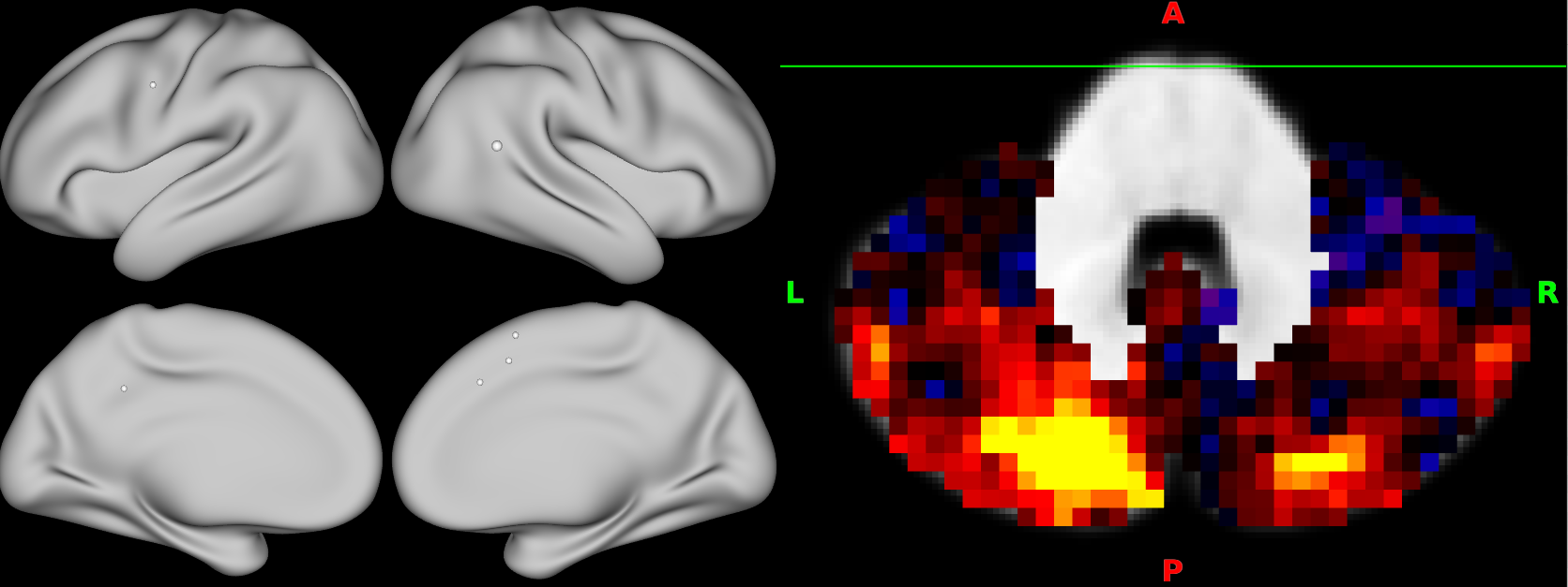
You can render pdconn files on the cortical surface, and select the row (cerebellar voxel) by clicking on the volume display.
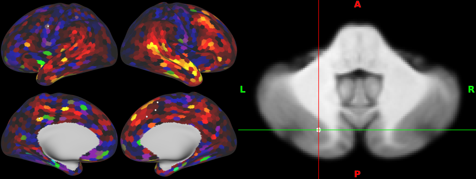
Vice versa, you can render dpconn files in the cerebellar volume, and select the row (cortical parcel) by clicking on the surface display.
Example: Extracting condition names from dscalar.nii files
Lets say you have a dscalar.nii file and you want to extract the condition names (found within the row axis).
Load your dscalar.nii with nibabel
import nibabel as nb
cifti_file = nb.load('path_to_your_cifti_file.dscalar.nii')
Access the nifti file header which contains information about the two axis:
cifti_file.header
You can get the axis you are interested in by indexing it. In our case we want the row axis so we index ‘0’:
axis = cifti_file.header.get_axis(0)
Finally, you can get an array of strings representing your conditions:
my_conditions = axis.name
Output:
array(['NoGo', 'Go', 'ToM', 'VideoAct', 'VideoKnots', 'UnpleasantScenes',
       'PleasantScenes', 'Math', 'DigitJudgement', 'CheckerBoard',
       'SadFaces', 'HappyFaces', 'IntervalTiming', 'MotorImagery',
       'FingerSimple', 'FingerSeq', 'Verbal0Back', 'Verbal2Back',
       'Object0Back', 'Object2Back', 'SpatialNavigation', 'StroopIncon',
       'StroopCon', 'VerbGen', 'WordRead', 'VisualSearchSmall',
       'VisualSearchMed', 'VisualSearchLarge', 'rest'], dtype='<U17')
Example: Plotting Cerebellar flatmaps of dscalar.nii files for conditions
What if you want to plot cerebellar flatmap of a specific condition in your dscalar.nii?
To do that, we will use 3 additional libraries (numpy, nitools and SUITPy).
-
Nitools will be used for extracting volumetric data from our CIFTI: https://nitools.readthedocs.io/en/latest/
-
SUITPy will be used to project Volumetric data to a Cereballar flatmap: https://suitpy.readthedocs.io/en/latest/
Say you are interested in plotting a flatmap for the ‘VerbGen’ task:
import numpy as np
import nibabel as nb
import nitools as nt
import SUITPy.flatmap as flatmap

task_of_interest = 'VerbGen'

# Load CIFTI
cifti_file = nb.load('path_to_your_cifti_file.dscalar.nii')

# Extract volume
volumetric_data = nt.volume_from_cifti(cifti_data)

# Project onto cerebellar flatmap
flatmap_img_data = flatmap.vol_to_surf(volumetric_data)

# Find the index of the VerbGen task using the header
index_of_task = np.where(scalar_axis.name == task_of_interest)[0][0]

# Plot
flatmap.plot(data= flatmap_img_data[:,index_of_task], cmap='autumn', \
    cscale=[-0.1,0.1],\
    new_figure=True, \
    colorbar=True, \
    render='matplotlib')